Where a Microsecond Goes: An Order's Path to CME


Trading infrastructure providers, including us, quote a single latency number. This post covers what slows an order down, what each stage of our path costs, what published measurements show for network and exchange delays, and what the number leaves out. Distance sets part of the delay; engineering and software choices set the rest.
The numbers at a glance
| Interval | Typical | Source |
|---|---|---|
| Order-to-wire: order handoff to our NIC | ~1 µs | Nanoconda |
| Wire-to-wire in our server, excluding strategy | 2.5–3 µs | Nanoconda |
| Our server to CME switching | ~500 ns each way | Nanoconda |
| CME GLink switching in Aurora | 3 µs each way, nominal | CME |
The order-to-wire stages add up to 0.65–1.5 µs; about 1 µs is typical.
CME's order handling and the return trip come on top. The sections below explain each row and what it leaves out.
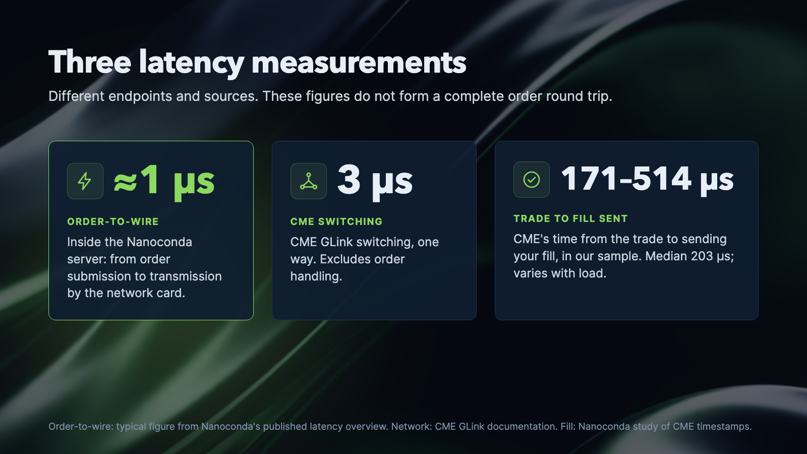
Outside the path we control: on the exchange side, CME's private fill messages showed a median of 203 µs from transaction time to sending time in our sample (CME Trade Summary vs iLink Latency). This is CME's own processing, so no provider can reduce it, but it shows where much of the time goes.
Where the delays occur and how to measure them
Several delays add up for a trading strategy: market data reaching the strategy, the strategy deciding, the order passing risk checks and the gateway, network travel to the exchange, and the exchange processing the order and replying. On a remote connection, distance adds a delay you cannot avoid. Once you are colocated, host processing, exchange handling, and occasional spikes matter more. Before optimizing anything, measure where the time goes and how much delay your strategy can tolerate before execution results get worse.
Every measurement needs a start event and an end event. We use the trading server's network card as the boundary: before it is processing inside the server, after it is network travel.
- Tick-to-trade runs from market data reaching the server's network card to the resulting order leaving it. It includes processing the data, the strategy's decision, and order-to-wire.
- Order-to-wire is the last part of tick-to-trade: from the strategy handing off an order to the network card sending it. It covers the local order path, including risk checks and the gateway.
- Order round trip, as we use it here, runs from the strategy handing off an order to the exchange's acknowledgement reaching the server's network card. It is order-to-wire plus network travel to the exchange, exchange handling, and the response's journey back. It leaves out market-data processing and the strategy decision.Some benchmarks start the round trip when the network card sends the order, so their figures leave out order-to-wire. Time until a fill is a different interval: it can include waiting for a matching order on top of processing and network delay.
Read each row in the table with its endpoints, statistic, and source in mind: half a round trip is not a measured one-way delay, and a median says nothing about the slowest responses.
| Measurement | Time | Ref |
|---|---|---|
| Human perception (for scale) | ||
| Visual reaction time, study mean, corrected for equipment delay (2015) | 213 ms | [1] |
| Internet routing | ||
| Verizon North American backbone, round trip, monthly mean (Aug 2026) | 36 ms | [2] |
| Trading-route links | ||
| Spread Networks fiber, Chicago–New York, round trip (2012 claim) | 12.98 ms | [3]† |
| McKay microwave via Quincy Data, Aurora–Carteret market data, one way (2016 claim) | 3.982 ms | [4]† |
| Remote link to CME | ||
| Fiber, 350 E Cermak (Chicago) to CME in Aurora, one way, Databento estimate | ≥287 µs | [5] |
| Nanoconda (for comparison) | ||
| Order-to-wire, typical | 1 µs | ‡ |
| Hardware and silicon (for scale) | ||
| Main-memory access, approximate | 100 ns | [9] |
| Cisco Nexus 3550-F switch, port to port, documentation example | 95 ns median; 107 ns max | [10]† |
| L1 cache access, approximate | 0.5 ns | [11] |
| Market structure (competitive context) | ||
| ES futures vs SPY ETF arbitrage window, median (2011) | 7 ms | [12] |
| LSE trading race, most common duration (2015 data) | 5–10 µs | [13] |
Memory and cache values are approximate scale figures, not measurements of a specific server; the main-memory figure is from a 2017 CACM article, the L1 figure from an older reference. The switch figures come from the mux-firmware documentation example; 107 ns is an observed maximum, not a guarantee. A trading race runs from the first successful request to the first failed competing one. † Provider-reported figures. ‡ Nanoconda's published typical figure.
Distance
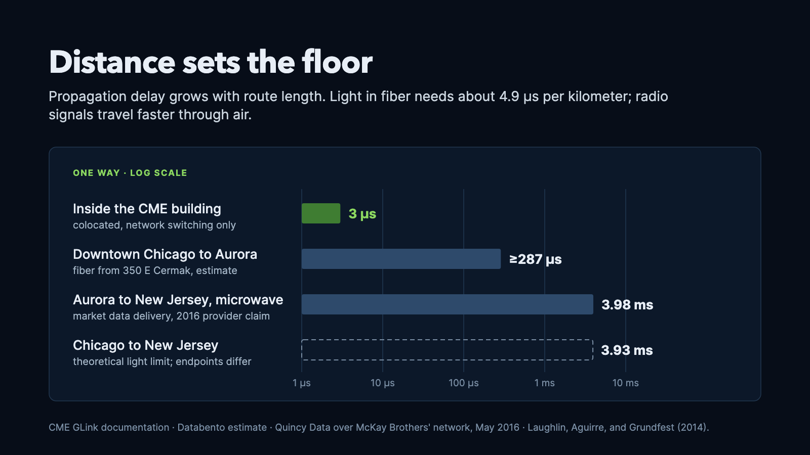
Light in standard single-mode fiber travels a kilometer in about 4.9 microseconds (refractive index about 1.47), or about 7.9 µs per mile. The delay grows with the length of the fiber. Radio through air is faster than light through glass, which made microwave attractive for latency-sensitive links between Chicago and New Jersey: chains of towers pass signals in straight lines through the air instead of through a cable. A study of Chicago–New York communication links measured how fast New York prices reacted to Chicago futures and found one-way time fell by 3 ms, first from a shorter, straighter fiber cable and then from microwave networks.
CME's matching engines run in its Aurora, Illinois, colocation facility. Fiber from the 350 E Cermak carrier hotel in downtown Chicago to Aurora adds a one-way delay of at least 287 µs, according to an estimate in a Databento blog post. Colocation puts your server in the same data center as CME's matching engines, with equidistant GLink access. The network from the Nanoconda server to CME's switching takes about 500 ns each direction (about 1.0 µs round trip). CME's own latency comes on top, because orders then cross CME's internal network before they reach its order-processing systems. CME gives a nominal 3 µs one-way delay for Aurora GLink's spine-and-leaf switching.
Host software
Once the strategy is colocated, the host's processing path becomes a larger part of the latency you control. To choose a networking stack, compare stacks on the same hardware. AMD's October 2025 white paper reports 80% lower latency with Onload than with Linux kernel TCP in a 4-byte sfnt-pingpong test on EPYC 9375F processors and X3522 adapters. The gain applies to networking only, so the effect on a full trading path depends on how much of that path is networking.
If networking is a large part of your delay, test kernel bypass. Onload runs on Linux and can speed up an application that uses standard sockets.
Market data and orders also wait when other tasks compete for the CPU. In a 2026 test, 99.9% of Linux request/response round trips finished within 19 µs (P99.9) with one thread running alone. With 48 threads competing for one core, it went above a millisecond. Assigning dedicated CPU cores to market data and order processing reduces competition with other work on the server.
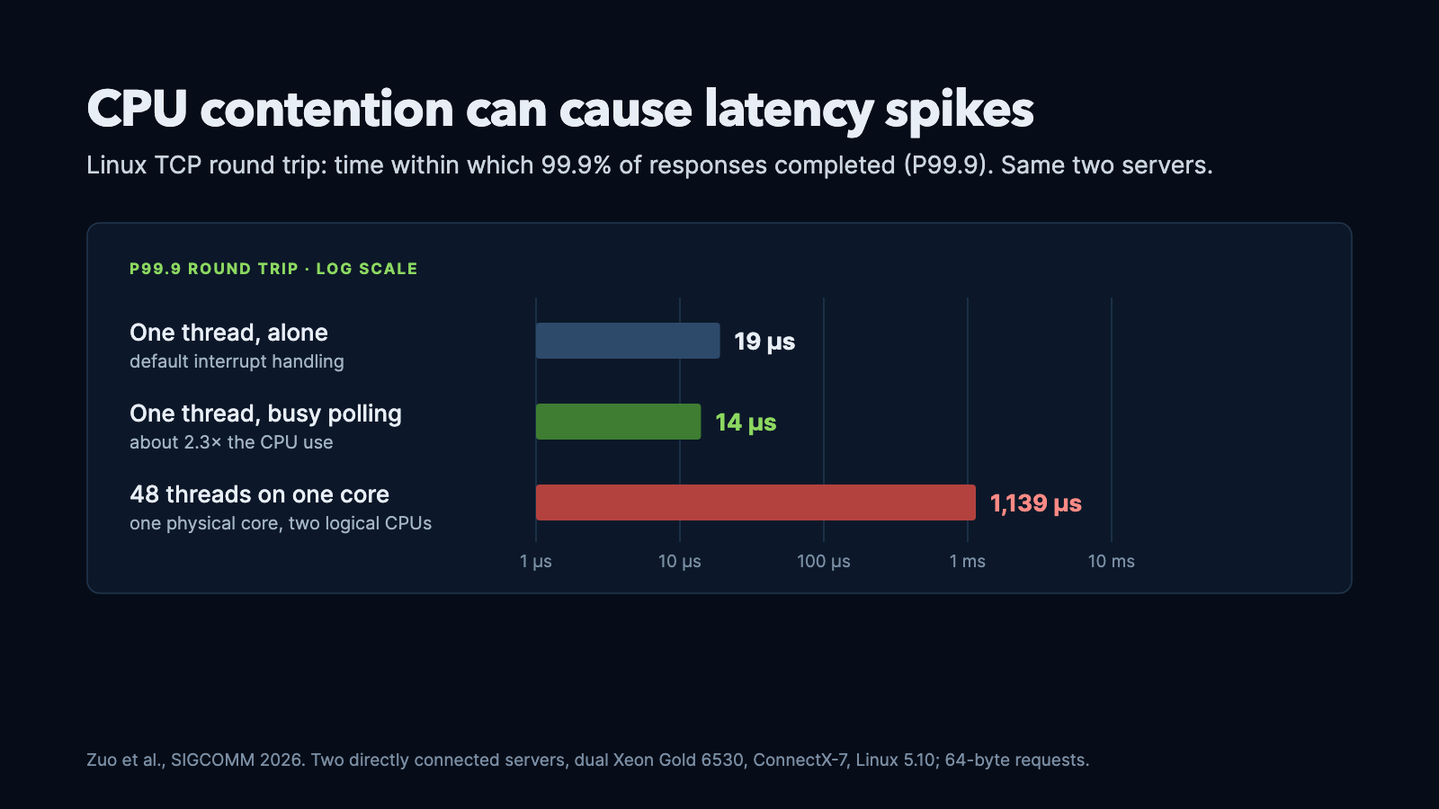
The way the application receives packets also affects latency. Polling (repeatedly checking for packets instead of waiting for an interrupt) brought P99.9 down to about 14 µs in the same test.
Tuning narrows the gap: in a 2025 comparison of six TCP stacks, tuned Linux had a median round trip of 17 µs against 13 µs for Demikernel, the fastest bypass stack tested (small requests, one connection, no competing traffic).
Running the strategy, risk checks, and gateway on separate machines adds network trips; even on one machine, moving data between cores takes time, so keep handoffs to a minimum.
Reducing latency spikes on the trading server
Kernel bypass reduces the work of sending and receiving packets, but Linux still schedules threads, manages memory, and runs other system work. Server tuning keeps that activity away from market-data and order processing. On Nanoconda's managed servers we handle this for you. If you run your own server, these are the main settings:
- Scheduler and timers.
isolcpusremoves selected cores from normal scheduler load balancing; you assign trading threads to them yourself.nohz_fullstops scheduling ticks under certain conditions, such as a single runnable task on the CPU, andrcu_nocbsoffloads RCU callbacks. - Idle and frequency. Each CPU idle state has a worst-case exit latency. Limit idle depth per CPU in sysfs, through the power-management QoS interface, or at boot with options such as
intel_idle.max_cstate. A performance frequency policy keeps clocks high but does not by itself keep the CPU out of deep idle. The kernel docs callidle=polldrastic. - Interrupts and background work. Move device interrupts (
/proc/irq/*/smp_affinity_list), kernel threads, and workqueues (cpumask) to a housekeeping core, then watch/proc/interruptsunder trading load to confirm the trading cores receive none. - Memory. Benchmark explicit and transparent huge pages; Hudson River Trading's huge-page guide explains the trade-offs. Keep memory resident with
mlockall, pre-touch the working set, and avoid copy-on-write faults. - SMT and NUMA. Test turning SMT off or keeping other threads off trading cores, and test CPU and memory placement, automatic NUMA balancing, and memory deduplication with your workload.
Measure the result. In one Linux tuning guide, a jitter tool showed a maximum of about 18 µs on the isolated core and about 17 ms on core 0; at the 99.9th percentile, about 4.9 µs and 6.6 ms. In a 30-second test, the two tuned CPUs got 3 and 4 timer interrupts; CPU 0 got more than 31,000. These are single runs on unspecified hardware.
When you evaluate a provider, ask for measured latency and tail figures from the deployed setup and how they were tested.
Nanoconda design: one machine, no network hops between components
You build and test your strategy on your own machine, then deploy it to an isolated, dedicated container in the managed colocated environment. Where the product includes SSH access, you install, start, stop, and manage your application in the container yourself. The container runs on the same server as the feed handler, risk checks, and order gateway. Nanoconda runs the exchange gateways; you run your strategy.
Your application links the Nanoconda library and works with these components through shared memory. The container has no direct access to the exchange-facing network interfaces. Because the strategy runs on this server, there is no network trip to a remote strategy machine between market data and order.
CME systems
    │ Market data
    ▼
Colocated server running your strategy and Nanoconda services
    NIC → Feed handler → Shared memory → Your strategy (in your container)
    Your strategy → Shared memory → Risk checks → Order gateway → NIC
                                                                  │ Order
                                                                  ▼
                                                             CME systems
Kernel bypass on both ends. The feed handler receives market data through ef_vi, and orders go out through TCPDirect, AMD's kernel-bypass TCP/UDP implementation for Solarflare adapters. AMD describes it as lower latency than Onload, with fewer features and a different API.
Shared memory between components. The strategy reads market data and submits orders through a shared memory region. It avoids a network trip, but polling, buffering, and moving data between CPU cores add some latency.
Risk on the same server. Pre-trade checks run in the local order path, so there is no trip to a separate risk server in this setup.
Dedicated CPU cores. The API lets you assign market-data and account-update callbacks to specific CPU cores, with background work kept on other cores, to reduce CPU competition and latency spikes. Shared hardware can cause delays.
The timings in this article are for the local shared-memory path. GUI, Remote API, FIX, and Sierra Chart access use different interfaces; measure them separately.
Nanoconda: the send path, stage by stage
These are our typical figures for the time from a strategy's decision to the order leaving the network interface. They are for an optimized production deployment: CPU pinning, cache warming, dedicated trading cores, a tuned OS, and supported Solarflare/Xilinx hardware. Actual timings depend on hardware, CPU architecture, thread placement, cache state, and workload.
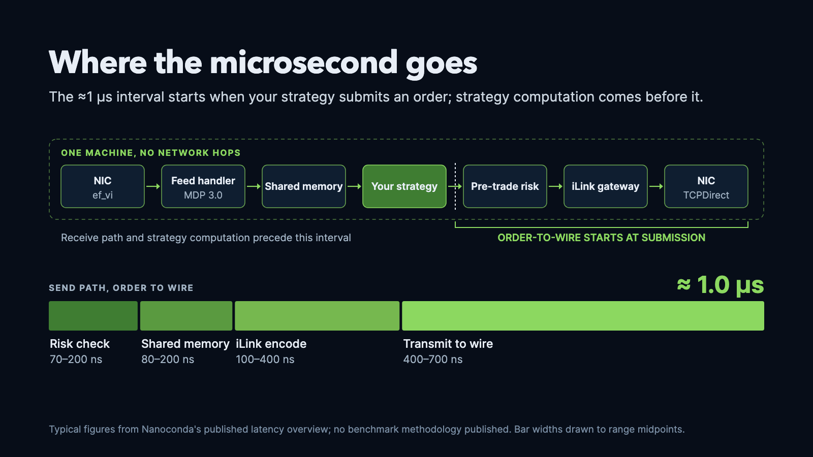
| Stage | Typical |
|---|---|
| In-memory pre-trade risk | 70–200 ns |
| Shared-memory transfer | 80–200 ns |
| iLink message normalization | 100–400 ns |
| TCPDirect / PCIe transfer | 400–700 ns |
| Order-to-wire, typical | ~1.0 µs (stages: 0.65–1.5 µs) |
The stage ranges are typical values, not percentiles, so their sum is not the range or tail of the total.
Nanoconda: the receive path
The receive path moves data from the NIC, parses CME MDP 3.0 messages, and makes the result available through shared memory. Nanoconda's feed-handler documentation describes configurable ingestion and processing threads, so thread placement and configuration affect this path's latency.
Our typical figures for this path run from market data reaching the network card to the data being available to the strategy.
| Stage | Typical |
|---|---|
| Solarflare EFVI / PCIe transfer | 500–700 ns |
| CME MDP 3.0 message parsing | 200–400 ns |
| Shared-memory transfer (cross-core) | 300–400 ns |
| Receive path, typical | stages: 1.0–1.5 µs |
Together, the two paths give a typical wire-to-wire time inside the server of 2.5–3.0 µs, a conservative figure: the stages add up to 1.65–3.0 µs. It excludes the strategy's own computation and the exchange round trip.
| Part of wire-to-wire | Stages |
|---|---|
| Software processing | 0.75–1.6 µs |
| EFVI/TCPDirect PCIe transfer (500–700 ns receive, 400–700 ns send) | 0.9–1.4 µs |
The transfer stages are the largest listed contribution; this breakdown does not isolate which part comes from software, PCIe, or the NIC.
How much speed does your strategy need?
Lower latency helps when your order has to arrive before a competing order or a price change. How soon depends on how the strategy trades.
Reacting across markets. A move in one instrument can change the value of another; a futures move, for example, can mean an ETF quote needs to change. Futures–ETF arbitrage trades a temporary mismatch between CME E-mini S&P 500 futures and SPY, as examined in a study of cross-market arbitrage. The link between venues affects this too: a study of Chicago–New York microwave links found that weather disruptions delayed New York equities' reaction to Chicago futures by about 2 ms. Colocating at the exchange where you send orders shortens the route to the exchange, but the signal has to travel from its source first, so fast cross-market strategies depend on both server placement and the link between venues.
Competing for queue position. Spread-focused market makers place buy and sell limit orders to earn the bid–ask spread. When several traders quote the same price, arriving first can raise the chance of a fill where the exchange uses time priority. A model of queue-position value looks at the balance between earning the spread, getting filled, and trading against better-informed counterparties. CME's matching algorithms include FIFO, pro-rata, and mixes of the two, so the value of arriving first depends on the contract. Colocation removes the long external trip; once competitors are nearby too, differences in local processing and order submission can decide queue position at the microsecond level. Even with a good queue position, a fill depends on incoming orders and the matching rules.
Updating or canceling quotes. Market makers also adjust quotes as prices and inventory change. A market-making model with inventory risk shows how a trader's holdings affect the prices it is willing to quote. When new information changes what a quote is worth, the market maker may need to cancel it quickly. The race is between the cancel and an order that could trade against the old price. Research on speed in liquidity provision explains how faster cancels help liquidity providers avoid trading at stale prices. Market data, quote decisions, and the cancel path all need to be consistently fast: occasional long delays can hurt even when average latency is low.
Trading signals with more time to act. Another kind of spread strategy trades mean reversion: an expected return to a normal price relationship. A study of mean-reverting energy futures spreads, for example, tests positions across expiry months of crude oil and natural gas futures using settlement prices. If your signal stays useful for seconds, minutes, or longer, and a few extra milliseconds barely change your results, microsecond-level optimization may offer little benefit. Faster access can improve an entry, exit, or hedge; size the infrastructure to the measured benefit. A server near the exchange may be enough; strategies racing for immediate price changes or queue position have a stronger case for exchange colocation.
To find out how much latency your strategy can tolerate, add market-data, order, and cancel delays one at a time in replay or simulation and compare fills, prices, and execution costs. The results show whether a shorter network route, faster local processing, or fewer latency spikes would help most.
Measure it yourself
Measure the whole path your strategy depends on. Local infrastructure timings leave out strategy computation, network travel, exchange processing, and any wait for a fill. Test under realistic load and report slow responses as well as typical values.
You can check live session latency in two ways: the web portal shows a latency histogram and breakdown, and the latencyreport app in the Nanoconda CLI prints a latency report as CSV:
nanoconda-cli -a latencyreport -c market-access-config.xml
Use your session's configuration file.
The Order Entry API and Market Data API expose timestamp members such as writetime and receivetime. For live receive-path latency, subtract receivetime from writetime. With efvi-hw-timestamps enabled, receivetime holds the EFVI hardware timestamp (feed-handler documentation). Both timestamps are taken on the same server, and the NIC clock is PTP-synchronized with the system clock, so the two can be subtracted.
Host intervals can be measured with calibrated software clocks or with hardware timestamps at the card, as long as the boundary is stated. A network round trip uses one clock. One-way measurements across machines need synchronized clocks and a stated synchronization error.
The 203 µs exchange-side figure above is CME's sending time minus transaction time, from our sample. CME's timestamp overview explains the measurement points, and its iLink and MDP specifications define TransactTime, SendingTimeEpoch, and SendingTime. It is not the time until your server receives a fill.
For a result others can reproduce, record the hardware, software version, configuration, workload, and timestamp boundaries. Report the median and tail percentiles with sample counts, and measure strategy processing separately if you are after tick-to-trade.
References
- Woods, Wyma, Yund, Herron, and Reed, "Factors influencing the latency of simple reaction time," Frontiers in Human Neuroscience, 2015.
- Verizon IP latency statistics, August 2026 monthly average.
- Spread Networks, Chicago–New York latency improvements, 4 October 2012 — historical 12.98 ms dark-fiber round-trip provider claim.
- Quincy Data, latency reductions with McKay Brothers upgrades, 12 May 2016 — historical 3.982 ms one-way Aurora–Carteret market data delivery claim over McKay's microwave radio network; not a round-trip measurement.
- Databento, "Where is the CME matching engine located?".
- Nanoconda, "CME Trade Summary vs iLink Latency".
- CME Group, GLink Architecture — Aurora — nominal 3 µs one-way for spine-and-leaf switching only; excludes order handling and is not a cross-connect cable measurement.
- Zuo, Hwang, Tang, Agarwal, and Cai, "Understanding Host Network Stack Latency," SIGCOMM 2026.
- Barroso, Marty, Patterson, and Ranganathan, "Attack of the Killer Microseconds," Communications of the ACM 60(4), 48–54, 2017 — Table 1 gives approximate latency scales, including 100 ns memory access; not a measurement of current production hardware.
- Cisco Nexus 3550-F latency statistics — example switch readout included for scale, not a guaranteed latency specification.
- Peter Norvig, "Teach Yourself Programming in Ten Years," approximate operation timings — approximate memory and cache values included for scale, not measurements of current trading hardware.
- Budish, Cramton, and Shim, "The High-Frequency Trading Arms Race," QJE 2015.
- Aquilina, Budish, and O'Neill, "Quantifying the High-Frequency Trading Arms Race," QJE 2022.
- Laughlin, Aguirre, and Grundfest, "Information Transmission Between Financial Markets in Chicago and New York," Financial Review 49(2), 283–312, 2014. Open-access preprint.
- AMD, Low Latency Solutions with EPYC 9005 and Alveo X3, October 2025 — same-platform Linux TCP versus Onload communication benchmark.
- Awamoto and Honda, "Opening Up Kernel-Bypass TCP Stacks," USENIX ATC 2025, 249–262.
- Shkilko and Sokolov, "Every Cloud Has a Silver Lining: Fast Trading, Microwave Connectivity, and Trading Costs," Journal of Finance, 2020.
- Moallemi and Yuan, "A Model for Queue Position Valuation in a Limit Order Book," working paper, revised June 2017.
- CME Group, Matching Algorithm Overview.
- Avellaneda and Stoikov, "High-frequency trading in a limit order book," Quantitative Finance 8(3), 217–224, 2008. Free author-hosted copy.
- Baldauf and Mollner, "Fast traders make a quick buck: The role of speed in liquidity provision," Journal of Financial Markets, 58, 100621, 2021.
- Lubnau and Todorova, "Trading on mean-reversion in energy futures markets," Energy Economics 51, 312–319, 2015.
- CME Group, Globex Timestamps.
- CME Group, iLink Execution Report — Trade Outright, timestamp field definitions.
- CME Group, MDP 3.0 — SBE Technical Headers, SendingTime definition.